How unique is Hillary Clinton’s style? What does her speeches tell us about her uniqueness? In this post I built several Naive Bayes models, trained them on Hillary’s 2016 campaign speeches and applied them on other remarks, tweets and text corpuses. The results is Interesting, and presents another journalistic use-case for machine learning.

I sometimes have a hard time to find applications for machine learning in data journalism. While models can help to predict future data points upon past observations, sometimes there is simply not a great use-cases that would tell readers anything new. I am more hopeful when it comes to text analysis. Text is everywhere. Text is part of the presidential rally, and text is part of every journalist reporting about it. And there is also too much text data, for everyone to read and process. Here, the use of automated data analytics and machine learning could contribute great value and new meaningful insight. A start has been made with an earlier post.

Naive Bayes for text analysis

Here, I use machine learning to make a judgement on Hillary Clinton’s uniqueness. How? By using her 2016 campaign speeches from Clinton’s campaign website, by mixing it up with speeches from other US presidents (including some of her husband’s speeches), and by training a fairly simple Naive Bayes model by applying a “Bag of Words” methodology (here a good tutorial to follow), we can observe how easy for the computer model it is to filter out her speeches and comments from others.

In theory, if the model doesn’t preform well, Hillary Clinton’s speeches - including her words and phrases and topics - could be very similar to other political speakers. From here, we could judge her on for being not unique enough, and not able to voice her own though and words enough of the time (whatever that might mean). Many US voters these days, I am convinced value a presidential candidate who is herself, as we can see from the popularity of Donal Trump (who is all himself, in any speech or interview).

On the contrary, if the model doesn’t do well, I may either blame myself on wrongly calibrating the model, or blame the state of the text data collected. If we could provide evidence that Hillary Clinton’s speeches are unique enough - in the sense that the classifying model is doing well - we can proof that she is who she claims to be.

The catch

The approach has some hooks. As we only apply a bag of words methodology, the most frequent words have a greater impact on the classifier. The dates the speeches were delivered have not been taken into account either. Applying Naive Bayes (NB), has some additional drawbacks:

• While the Naive Bayes classifier is said to be fast, and very effective, able to deal with noisy and missing data and requests relatively few examples for training (it is easy to also obtain the estimated probability for a prediction),
• it relies on an often-faulty assumption of equally important and independent features. NB isn’t ideal for datasets with many numeric features and estimated probabilities are less reliable than the predicted classes.

I will run you through the process on how prepare text data and how to classify Hillary’s speeches and text documents. For this, we will look at how well NB can perform on text classification for the following:

• find her speeches in a pile mixed up with her husband’s Bill (Is she unique enough for the algorithm to spot hers?)
• Hillary’s own speeches from the time when she was Secretary of State (giving clues about whether she might have “changed her style” over the past years)
• and on Hillary’s recent tweets (could we spot which tweets she may not have written herself?)

Get the data:

To train a Naive Bayes model, we need text data. We fetch it from Hillary’s campaign website.

# Clinton 2016 speeches from Hillaryclinton.com:
library(xml2)
library(rvest)
library(dplyr)
library(tidyr)

url1 <- "https://www.hillaryclinton.com/speeches/page/"
get_linkt<- function (ur) {
  red_t <- read_html(ur)
  speech <- red_t %>%
    html_nodes(".o-post-no-img") %>%
    html_attr("href")
  return(paste0("https://www.hillaryclinton.com", speech, sep = ""))
}
df_clinton_2016 <- NULL
for (t in 1:10) {
  linkt <- paste0(url1, t, "/", sep = "")
  print(linkt)
  df_clinton_2016 <- rbind(df_clinton_2016, as.data.frame(get_linkt(linkt)))
}

getspe <- function (urs) {
  red_p <- read_html(urs)
  speech1 <- red_p %>%
    html_nodes(".s-wysiwyg") %>%
    html_text()
  as.character(speech1)
  wann <- red_p %>%
    html_node("time") %>%
    html_text()
  as.character(wann)
  dataframs <- cbind(as.data.frame(speech1), as.data.frame(wann))
  return(dataframs)
}

fin_2016 <- NULL
for (p in 1:nrow(df_clinton_2016)) {
  tryCatch({
    linkp <- df_clinton_2016[p, 1]
    print(linkp)
    fin_2016 <- rbind(fin_2016, as.data.frame(getspe(as.character(linkp))))
  }, error=function(e){cat("ERROR :",conditionMessage(e), "\n")})
}
get_speech_2016 <- function (u) {
    red_s <- read_html(u)
    speech <- red_s %>%
      html_nodes() %>%
      html_text()
    wann <- red_s %>%
      html_nodes() %>%
      html_text()
    wo <- red_s %>%
      html_nodes() %>%
      html_text()
    bingins <- cbind(as.data.frame(speech), as.data.frame(wann), as.data.frame(wo))
}

Is Hillary only a new Bill?

How different is her speech content from Bill Clinton’s. How unique are the messages she is sending out in her 2016 campaign speeches compared to her husband’s? First we will clean and then train and test the NB on a dataset that contains both Hillary’s and Bill’s speeches.

Text data fetching:

For each part of this post, we will both train the model, and then classify the test set, resulting in a judgement on how well the model does on the new data. For this we need our data to be clean. For demonstration purposes, we will do it here once, but skip over it later on.

First off, I used this website to scrape some of Bill Clinton’s speeches (Bill’s speeches might not be the best (e.g. speeches that occured at a different time maybe different by its nature, the topics he spoke about back then differ from today’s, and they differ in gender). However, they are living together. One might assume, that Bill may have rubbed off on Hillary after all those years. Let’s mix them up first with Hillary’s 2016 speeches:

ge_links <- function (x) {
  t <- read_html(x)
  linky <- t %>%
    html_nodes(".title a") %>%
    html_attr("href")
  return(paste0("http://millercenter.org", linky, sep = ""))
}

url_pre <- "http://millercenter.org/president/speeches"

df_pres <- NULL
df_pres <- rbind(df_pres, as.data.frame(paste0("", ge_links(url_pre), sep = "")))

######### change column with column id
names(df_pres)[1]<-"link"

View(df_pres)

get_speech_pres <- function (x) {
  t <- read_html(x)
  speech <- t %>%
    html_node("#transcript") %>%
    html_text()
  return(as.data.frame(speech))
}

get_speech_pres("http://millercenter.org/president/washington/speeches/speech-3459")

df_speeches2 <- NULL
for (y in 90:128) {
  print(y)
  tryCatch({
    link_y = as.character(df_pres[y, 1])
    df_speeches2 <- rbind(df_speeches2, (get_speech_pres(link_y)))
  }, error=function(e){cat("ERROR :",conditionMessage(e), "\n")})
}

# Build a common structure - type and text as columns:
Bills <- df_speeches2  # Bill's speeches
Bills <- Bills %>%
  mutate(type = "Bill") %>%
  mutate(text = speech) %>%
  select(-speech)

Hillary_2016 <-  fin_2016 # Hillary's speeches
Hillary_2016 <- Hillary_2016 %>% select(speech1) %>%
  mutate(type = "Hillary") %>%
  mutate(text = speech1) %>%
  select(-speech1)

# rbind them (concatenate them):
bill_hillary <- rbind(Hillary_2016, Bills)

# Mix them up - apply a random sampling function
nrow(final_clintons) # [1] 135
bill_hillary_random <- sample_n(bill_hillary, 135) # sample_n, a great dplyr function for random sampling

Clean the data:

To help with data cleaning, the text processing package ‘tm’ by Ingo Feinerer is of great help. To start things off, we need a corpus, a simple collection of text documents. We use the VCorpus() function in the tm package after we convert the features in the column type into the data format of type factor.

library(NLP)
library(tm)

# Convert type column into as.factor()
bill_hillary_random <- bill_hillary_random %>%
  mutate(type = factor(type))

# Check distributions:
prop.table(table(bill_hillary_random$type))

# 28% are Bills speeches, the rest are Hillary's
Bill   Hillary
0.2888889 0.7111111

We use the VectorSource() reader function to create a source object from the existing hil_bill$text vector, which can then be converted via VCorpus().

hil_bill_corpus <- VCorpus(VectorSource(bill_hillary_random$text))

# Check class:
class(hil_bill_corpus)  # [1] "VCorpus" "Corpus"

Think of the tm’s coprus object as a list. We can use the list operations to select documents in it and use inspect() with list operators to access text corpus elements.

Next we create a document-term matrix via tm. A document-term matrix or term-document matrix is a mathematical matrix that describes the frequency of terms that occur in a collection of documents. In a document-term matrix, rows correspond to documents in the collection and columns correspond to terms. We combine it with basic cleaning operations, via functions tm provides, excluding a custom stopwords function. The DocumentTermMatrix() function helps us to break up the text documents into words:

# Stop-words (and, or ... you get the point)
stopwords2 = function (t) {removeWords(t, stopwords())}
# test stopwords function:
stopwords2("He went here, and here, and here, or here") # [1] "He went ,  ,  ,  "


# DocumentTermMatrix
hil_bill_dtm <- DocumentTermMatrix(hil_bill_corpus, control = list(tolower = T, #  all lower case
                       removeNumbers = T, #  remove numbers
                       stopwords2 = T, #  stopwords function
                       removePunctuation = T, #  remove .
                       stemming = T,
                       # Stemming reduces each word to its root from. Imagine you have words in the corpus such as "deported" or "deporting". Appliing the function would result in "deport" only, stripping the suffix (ed, ing, s ...).
                       stripWhitespace = T
                       # removes whitespaces or reduces them to only one each
                       ))
hil_bill_dtm
                       Non-/sparse entries: 94330/1356110
                       Sparsity           : 93%
                       Maximal term length: 45
                       Weighting          : term frequency (tf)

Lets split the data up into the training and test data, and save the outputs (“Bill” or “Hillary”) as a separate dataframe

hil_bill_dtm_train <- hil_bill_dtm[1:80, ]
hil_bill_dtm_test <- hil_bill_dtm[81:135, ]

# Actual output - whether it was Bill's or Hillary's speech                        
hil_bill_train_labels <- bill_hillary_random[1:80, ]$type
hil_bill_test_labels <- bill_hillary_random[81:135, ]$type

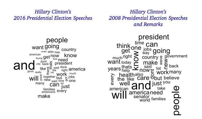
Now we have all the data in a clean form, allowing us to train our model. Lets visualise term frequencies via a wordcloud:

library(RColorBrewer)
library(wordcloud)
# filter the data for a word cloud
 hill <- subset(bill_hillary_random, type == "Hillary")
 bill <- subset(bill_hillary_random, type == "Bill")
 wordcloud(bill$text, max.words = 50, scale = c(3, 0.5)) # give us 50 most common words, you can do the same for Hillary's speeches

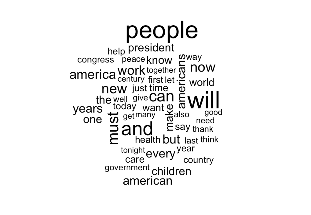
Classic Bill, he uses a set of disciplinary. For our model, we can reduce the number of words that are being taken into account as features for the model to words that appear more than a certain amount of times. Here we reducing it to at least 6 times. To do this, you can use the findFreqTerms() function by the tm package. Hereby we reduce the number of features down to only the ones that are making a major difference to the probability calculation in our model. Our feature set now consists of 1,674 features.

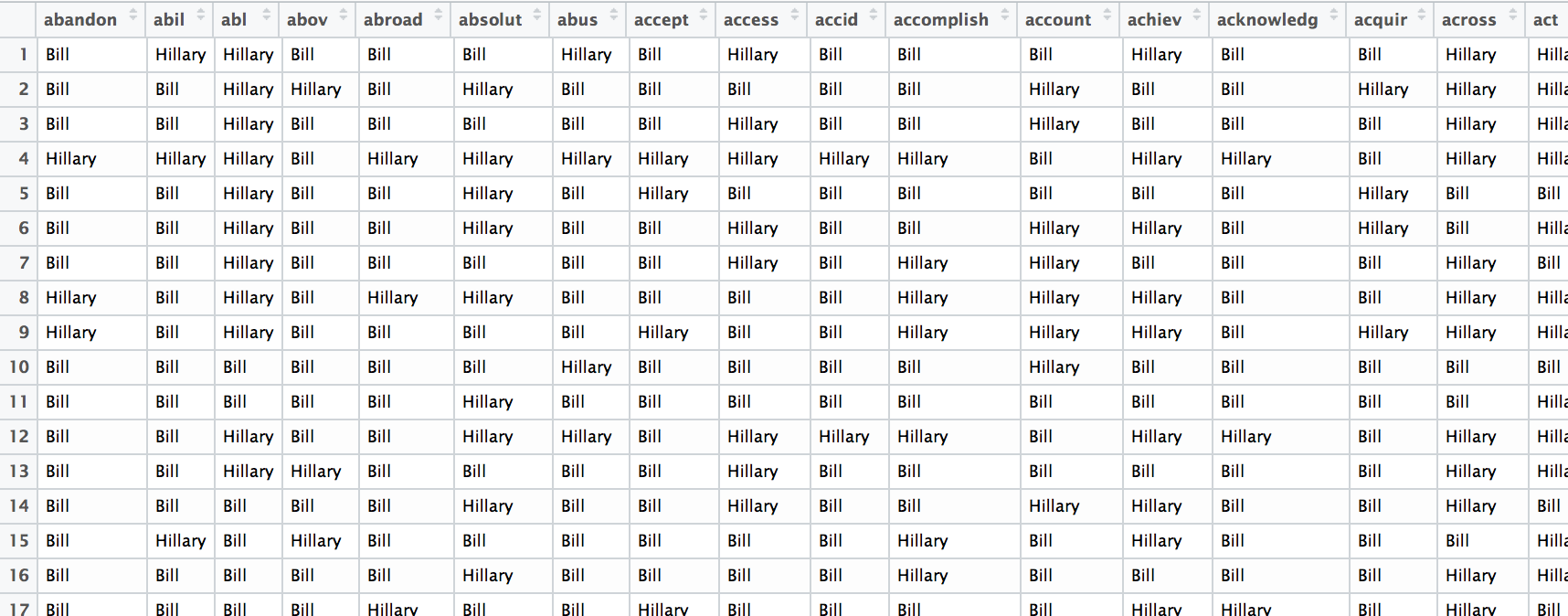
hil_bill_freq_words <- findFreqTerms(hil_bill_dtm_train, 12)
str(hil_bill_freq_words)
# show the structure
chr [1:1674] "abandon" "abil" "abl" "abov" "abroad" "absolut" "abus" "accept" "access" "accid" "accomplish" ...

Now the DocumentTermMatrix’s features, the words in the text documents (each speech), needs to be filtered according to the most frequent terms we just worked out via findFreqTerms(). We build a “convert” function to set categorical features to “Hillary” in case it is her speech document we are dealing with, otherwise it’s Bill’s. Lastly we convert it back to a data-frame.

# Filter most frequent terms appearing (for test and training data):
hil_bill_dtm_freq_train <- hil_bill_dtm_train[, hil_bill_freq_words]
hil_bill_dtm_freq_test <- hil_bill_dtm_test[, hil_bill_freq_words]

# the DTM needs to be filled now
convert_counts <- function (x) {
                              x <- if_else(x > 0, "Hillary", "Bill")
                              }
# Apply convert function to get categorial output values
hil_bill_train <- apply(hil_bill_dtm_freq_train, MARGIN = 2,
convert_counts)
hil_bill_test <- apply(hil_bill_dtm_freq_test, MARGIN = 2,
convert_counts)

#convert to df to see whats going on:
hil_bill_train_df <- as.data.frame(hil_bill_train)
View(hil_bill_train_df)

Training the model

Lets train a model by using the package e1071 to apply the naiveBayes() function.

# Train the model:
library(e1071)
library(gmodels)

hil_bill_classifier <- naiveBayes(hil_bill_train, hil_bill_train_labels, laplace = 0) # we set the laplace factor to 0

# Predict classification with test data:
hil_bill_test_pred <- predict(hil_bill_classifier, hil_bill_test)

# See how well model performed via a cross table:
CrossTable(hil_bill_test_pred, hil_bill_test_labels,
prop.chisq = F, prop.t = F,
dnn = c("Predicted", "Actual"))

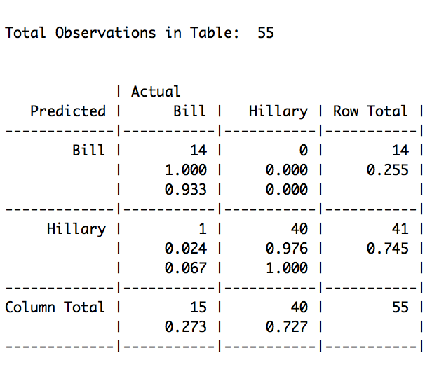
So above we did it.

The table reveals that in total, 1 out of 55 were miss-classified, or 0.018% percent of the speeches (1 that were actually Bills got miss-classified as Hillary’s, and 0 of Hillary’s got incorrectly classified as Bills). Naive Bayes is the standard for text classification.

Is this evidence enough? Probably not, but it’s a start. It may have proven the point that Hillary is unique enough in her 2016 speeches, compared to her husband’s back in the 90ties. What about other’s? How about Obama. He is much closer on the topics Hillary has to deal with today, than Bill was when he ran for 42nd president of the United States.

Obama vs. Hillary:

Lets try the same spiel with Obama’s speeches. We run the model on 107 of Hillary’s 2008 presidential campaign speeches and Hillary’s 96 2016 campaign speeches.

Hillary   Obama
  96       45

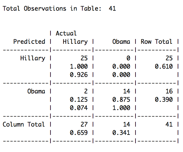
NB performs really well again, however not as well as before. With only a 4.87% of miss-classified instances, the model seems to be working reliably, and able to filter Hillary’s speeches from Obama’s. So neither Obama has massively influenced her’s speaking style.

Hillary vs. her former self:

We talked about time, and that is is a problem. While she might have lost the Democratic nomination to Barack Obama in 2008, she became Secretary of State. Leaving office after Obama’s first term, she undertook her own speaking engagements before announcing her second presidential run in the 2016 election. So in theory, we should be able to provide evidence whether or not there is a significant differences in her style when comparing speeches before her speaking engagement tours and now after? Lets try and experiment with Hillary’s past.

She successfully served as the 67th United States Secretary of State from 2009 to 2013. We will take her 2009 speeches and mix it with the ones for her current campaign.

library(NLP)
library(tm)
library(e1071)
library(dplyr)
library(gmodels)

# read in Clinton_2009 speeches (Info from the US state department), and clean it:
regex <- "^.*:"
Clinton_2009 <- read.csv("download/clinton_2009.csv", stringsAsFactors = F)
View(Clinton_2009_fin)
Clinton_2009_fin <- Clinton_2009 %>%
  filter(str_detect(years, "2009")) %>%
  filter(kind == "Remarks") %>%
  mutate(type = "Clinton_2009")  %>%
  select(-years, -kind, -title) %>%
  mutate(text = str_replace_all(text, "SECRETARY CLINTON", "")) %>%
  mutate(text = str_replace_all(text, "MODERATOR", "")) %>%
  mutate(text = str_replace_all(text, "QUESTION", "")) %>%
  mutate(text = str_replace_all(text, "^[^,]+\\s*", "")) %>% # use speech sample from the first comma onwards
  filter(nchar(text) > 10) # remove empty rows
final_clintons2 <- rbind(clinton, Clinton_2009_fin) # combine the data with Hillary's speeches in the code previously

# Randomize the sample:
set.seed(111) # set seed, to reproduce example
hil_old <- sample_n(final_clintons2, 499)
hil_old<- hil_old %>%
  mutate(type = factor(type))
table(hil_old$type) # we have 403 of clintons 2009 speeches, and almost 100 of her current campaign speeches:
# Clinton_2009      Hillary
#         403           96
hil_old_corpus <- VCorpus(VectorSource(hil_old$text))

# clean and DocumentTermMatrix:
hil_old_dtm <- DocumentTermMatrix(hil_old_corpus, control = list(tolower = T,
                                                                   removeNumbers = T,
                                                                   stopwords = T,
                                                                   removePunctuation = T,
                                                                   stemming = T,
                                                                   stripWhitespace = T
))
hil_old_dtm_train <- hil_old_dtm[1:400, ]
hil_old_dtm_test <- hil_old_dtm[401:499, ]
hil_old_train_labels <- hil_old[1:400, ]$type  
hil_old_test_labels <- hil_old[401:499, ]$type


# Model building:
hil_old_freq_words <- findFreqTerms(hil_old_dtm_train, 5) # features restricted to an appearance of at least 5 times

convert_counds <- function (x) {
  x <- if_else(x > 0, "Hillary_2016", "Hillary_2009")
}
hil_old_dtm_freq_train <- hil_old_dtm_train[, hil_old_freq_words]
hil_old_dtm_freq_test <- hil_old_dtm_test[, hil_old_freq_words]
hil_old_train <- apply(hil_old_dtm_freq_train, MARGIN = 2,
                        convert_counds)

hil_old_test <- apply(hil_old_dtm_freq_test, MARGIN = 2,
                       convert_counds)
hil_old_classifier <- naiveBayes(hil_old_train, hil_old_train_labels, laplace = 0)
str(hil_bill_classifier)
hil_old_test_pred <- predict(hil_old_classifier, hil_old_test)
CrossTable(hil_old_test_pred, hil_old_test_labels,
           prop.chisq = F, prop.t = F,
           dnn = c("Predicted", "Actual"))

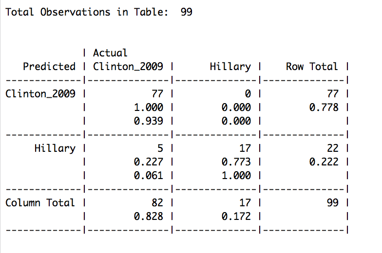
What we see, despite showing somewhat of the same terms (word-clouds below), the model guessed incorrectly in only about 5% of the cases, where Clinton’s 2009 remarks got miss-classified as 2016 speeches.

hill <- subset(hil_old, type == "Hillary")
Old_Hillary <- subset(hil_old, type == "Old_Hillary")
library(RColorBrewer)
library(wordcloud)
wordcloud(hill$text, max.words = 30, scal = c(3, 0.2))
wordcloud(Old_Hillary$text, max.words = 30, scale = c(3, 0.5))

Classifying Hillary’s presidential speeches (2008 vs. 2016)

The speeches as Secretary of State might not be perfect to judge on her campaign speaking style for the 2016 presidential election. To find a possibly more closely related dataset, Hillary’s presidential campaign speeches from her 2008 presidential election campaign might serve us well. Again, fetched data from the web, this time from the UCSB page . We see our model in action on the following instances:

Clinton_2008_Presidential_Election                       Hillary_2016
107                                 96

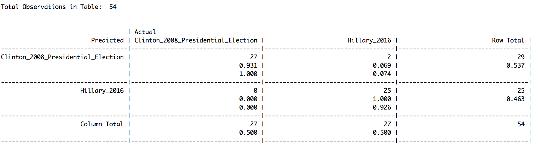Remarkable! Our NB model, with an accuracy of 98%, performed really well and was able to spot the differences between Clinton’s 2016 campaign and her campaign speeches she gave in 2007 and 2008. This could mean, that there is a significant difference between her speaking style and the topics she talks about, when comparing 2008 with 2016 campaign rally speeches.

Running the NB against Hillary’s tweets:

David Robinson has done it and found Trump’s uniqueness in his social media feed. We are looking at something similar for Hillary’s tweets.

In order to run a NB model against her tweets, we need text that Hillary didn’t write (as a training set). Her campaign blog may be a good start. I have written a scraper to get the last 100 blog entries. The data will be trained on 89 blog entries (cleaned up, so we don’t include Spanish entries here), and Hillary’s speeches of her 2016 campaign got included again representative for her own style. When we sort out the tweet messages that Hillary signs with an “-H” or “-Hillary”, we know they are hers (several people have reported in it, which we want to trust). With this in mind, we build a new model (as above). We take her blog posts, and her speeches, and train a NB model. Next, we build a test set with her tweets, and attach labels for the ones Hillary signed.

Classification on tweet text set

We run our classifier on the tweets and notice that our model got it completely wrong. How sad :-(

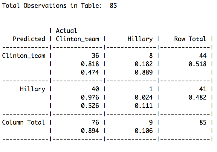
This could mean many things, including that the test data wasn’t properly cleaned. 47% were assigned to a wrong label, times when the model assumed that Hillary written the tweet herself, while for eight tweets by Hillary, the classifier reckoned that it was Clinton’s team who wrote it.

Conclusion:

Here is an overview on how well the model performed on various speakers and texts:

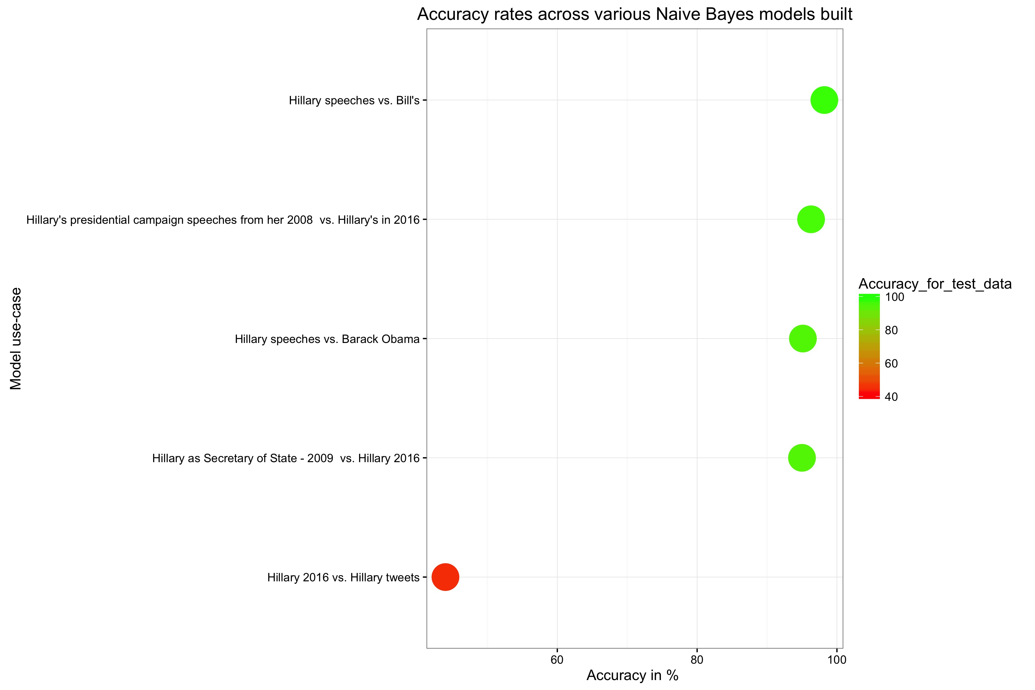Overall, Naive Bayes for text - in our case speech - classification is a powerful tool and works reliable in clean data. To judge how unique a person’s speaking style is works as long it is not being mixed up with written text data. Speeches are different from copy, and one doesn’t writes as one speaks. For Hillary’s tweets, this little experiment did not work.

However, our models could establish some evidence that showed that she is indeed her own persona. Her speeches may or may not reflect her own beliefs but certainly her own speaking style (and not her husband’s or other people she worked with in the past, such as Barack Obama). Her campaign is her unique voice, unique even in the sense of her past presidential rally in 2008.