What is the strategy to win the word’s biggest Skateboarding event this year, the 2016 SLS Nike SB Super Crown World Championship: A combination of run and best trick skills. An analysis on previous events and scores, with a data-driven judgement on who might have the best chances to win

Skateboarding has had a bad reputation for many years before Louis Vuitton used it in their ads. Today, skateboarding manages to get attention from all corners of the media landscape, and is now even only one step away to become an Olympic discipline. For decades, the typical competition format was that skaters were judged on their run, however Street league Skateboarding established a whole new data driven model to judge the performance of each street skater.

Instead of only being ranked on the run on the skate course, SLS introduced a real time rating system, single tricks evaluation, and a statistical evaluation of the scoring for each skater.

Sh.t is going down this weekend, at the Nike SB Super Crown World Championship

This Sunday, the biggest street skateboarding competition will take place in LA. SLS is the official street skateboarding world championship as recognized by the International Skateboarding Federation. At the recent Street League Skateboarding Nike SB World Tour in Newark, New Jersey, Nyjah Huston won the game and is now defending the 2015 SLS Championship title. Could we yield some interesting findings that could support skaters with empirical evidence how to win it?

Via a simple EDA, we will try to establish a number of relevant patterns gained from previous SLS results.

Relationships

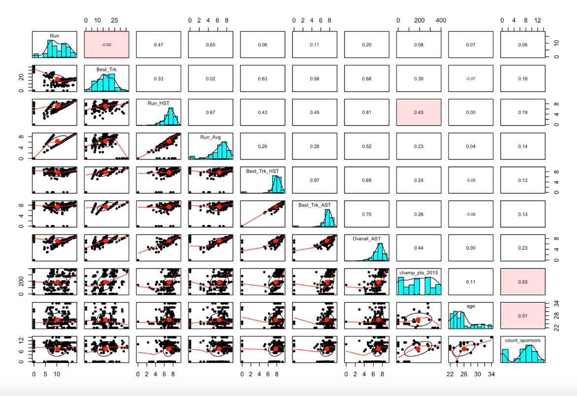
We understand from the correlation plot that there is a negative relationship between best-trick and run scores (-0.5), and an interesting one between age of skater and number of sponsors for each skater. Number of sponsors also plays nicely with final results for 2015 championship points.

Strategy

Loess line seems to draw a different picture, than the linear regression line. We will consider the structure later, when building a prediction model.

SLS’s competition format requires a lot more strategic planning today, than in the previous single score run-based competitions. An analysis of run-section and best-trick scores across recent Street League contests suggests that if players do perform well on either one of the sections, they usually perform not not as well in the other one (although, the linear trend is more significant for the preliminaries).

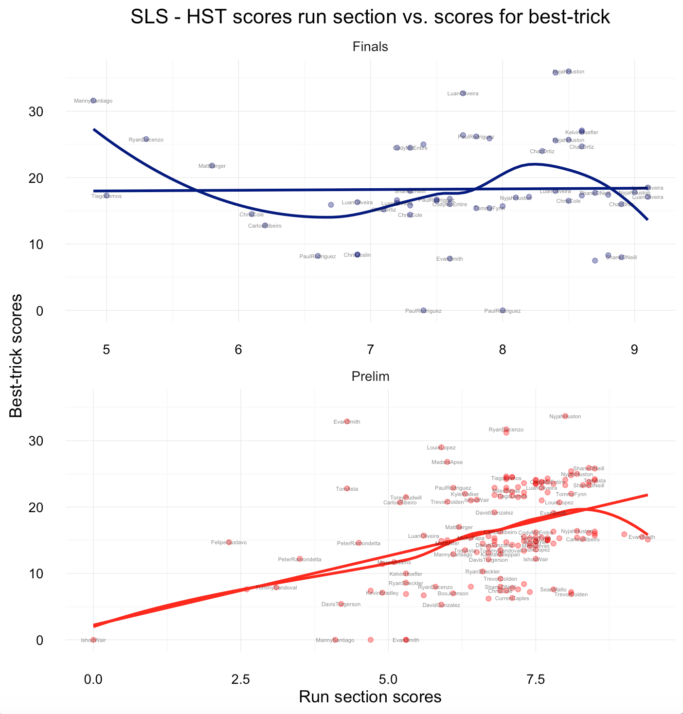
Chaz Ortiz and Shane O’Neill know how to perform well in the run section (mainly due to their vast experience in conventional skate contests), while Kevin Hoefler and Manny Santiago do well in the best-trick section. All-rounders such as Nyjah Huston and Luan Oliveira seem to do well in both sections for the finals. For the preliminaries, Shane and Nyjah leading the field, and are able to make it into the finals every single time.

Street League’s evolution

Launched in 2010, Street League Skateboarding is now an international competitive series in professional skateboarding. The SLS ISX, which is the core of the concept, is best described as a real time scoring system, allowing to include each trick independently. This stands in contrast to all other professional contests that judge on overall impression of a full run or series of tricks performed within a certain time frame. Because the outcome could change to the very last trick, the audience is kept in their seats. Transparency is high too. If the audience is able to understand how and why the skaters were judged the way they were, it adds an additional kick. To win, skaters are required to to have a strategy and be smart about how they play their skills and their endurance.

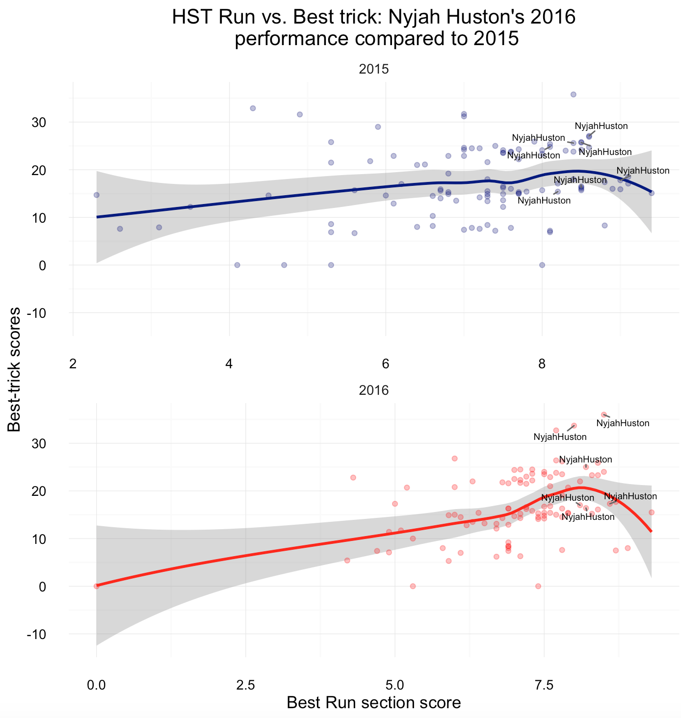
Comparing 2015 with 2016, Nyjah Huston’s run scores dropped slightly (this could be due to the fact that the scoring changed overall).

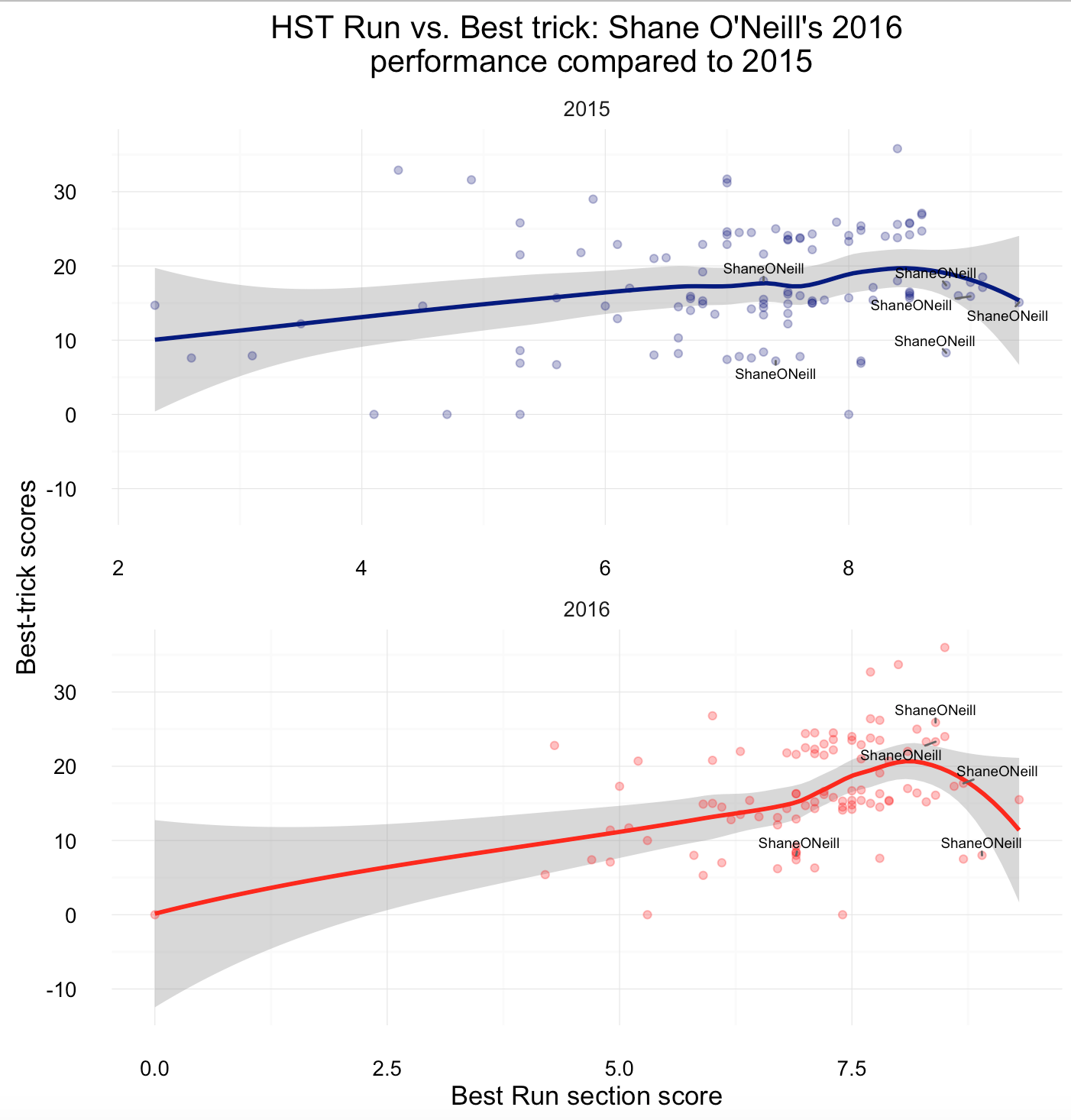
While Shane O’Neill could not improve on his highest run scores (but on best trick scores)…

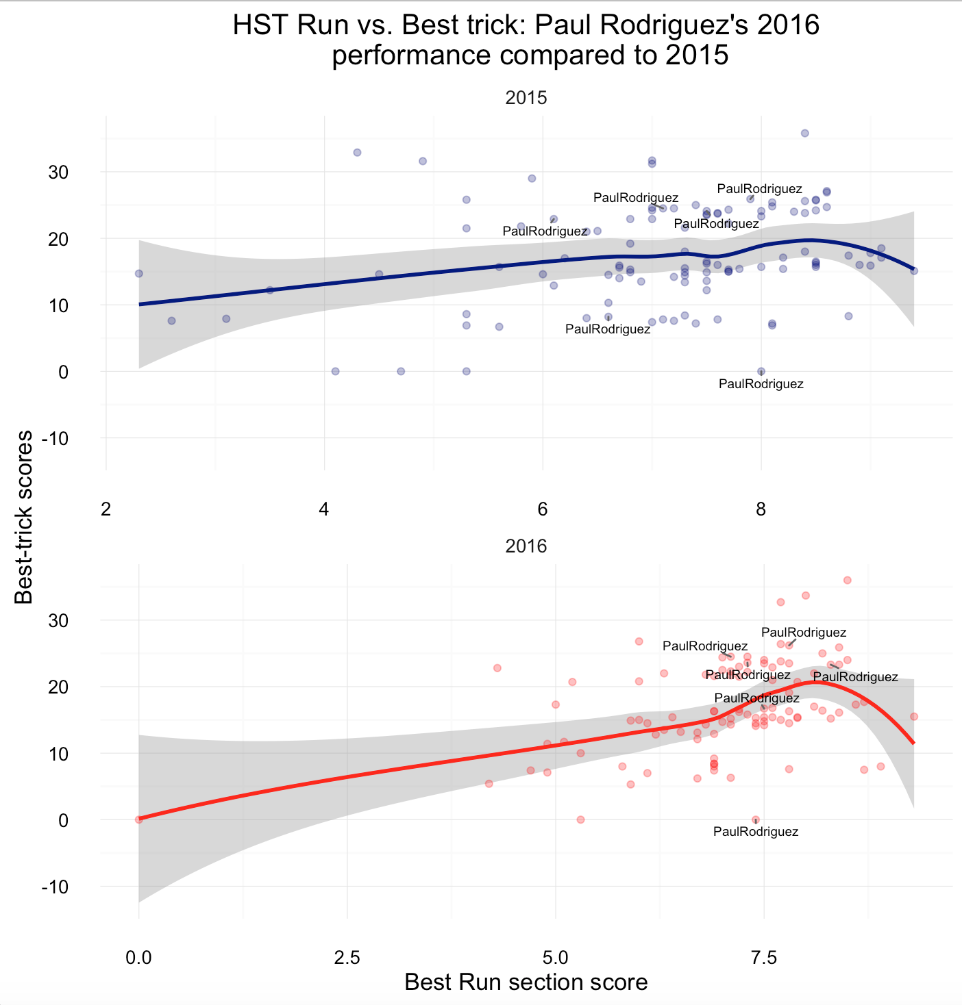
…Paul Rodriguez kept performing well across both sections.

If a skater is strikingly good at the run section, but fails to succeed in the best trick section (or vice versa), he (or she, female Street League was introduced in 2015) is unlikely to win.

So what is the best strategy? To answer the question, it helps to look at statistical coefficients and relationships for data points for the previous events.

Can you predict win probabilities after the run section?

Ok, we learned something from a basic exploratory data analysis. It’s time to shift our attention to machine learning and use what we learned.

Every SLS game starts with the run section, and ends with the best trick category. We could use machine learning and train one or multiple models to yield win probabilities after the run section, but before the best trick section and announcement of a winner to predict the winner.

In the next part our goal is to build multiple models, the practice to statistically compare them, and to come up with one that allows us to predict mid-game, which skater has the best changes to win the upcoming SLS Nike SB Super Crown World Championship.

Defining Independent and dependent variables

The outcome variable we will predict is a win or no-win. An variation to this is building a classification models on podium winners (1st, 2nd, 3rd). In different corner of the SLS website, we find information on the pro skaters, their previous performances and event-specific results.

From the SLS website, we scrape the number of 9 club scores for each skater (9 Club tricks are the most extraordinary moments in Street League and represents the highest scores in previous contest). 9 club scores may also be an important predictor on how well the players did perform in the best trick section.

Run HST and Run Avg may be important predictors to our models. Championship Points allow new and established skaters to qualify into the SLS Nike SB Super Crown World Championship. Each skater’s point score will be fed to our model.

We also throw in additional parameters. We have access to the age of some of the established pro skaters (the average age of pros is around 25, but outliers such as Cole may skew it), we know their stance (goofy or regular), and in the process of scraping and cleaning, I was able to count the number of sponsors.

Model types

We will build logic regression classification models, and compare how well they are able to perform against each other.

Logic Regression

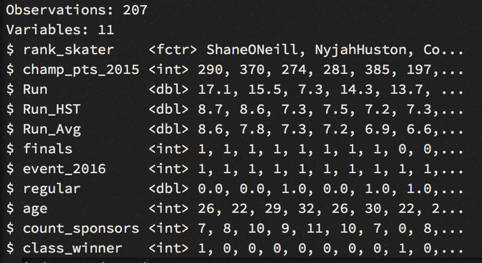
We will build and test a binomial logistic regression (our outcome variable which can assume 2 values). The following variables will be used to fit a GLM model in R:

# Overview of variables:
glimpse(win)

In a hidden process, I have cleaned the data, and converted them to required class types. Categorical data are factor values, while numerical are encoded as numerical or as an integer class. The age variable has no missing values anymore (removal of NA values in R), and they have been replaced with the average age values. Similarly, I dealt with the values in the stance column (to what degree this is valid, needs to be evaluated, but for now, we don’t care too much about stance - in theory, it shouldn’t make a difference whether a brilliant skater is goofy or regular).

# randomize, sample training and test set:
set.seed(10)
win_r <- sample_n(win, 207)

train <- win_r[1:150,]
test <- win_r[151:207,]

# fit GLM model:
model <- glm(class_winner ~.,family=binomial(link='logit'),data=train)
summary(model)

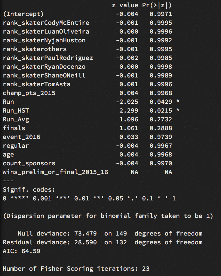
We learn from the summary function that most of the variables are not statistically significant for our model. Run_HST is possibly the best predictor we can use at this stage. A positive coefficient for Run_HST suggests - if other variables are kept equal - that a unit increase in highest run section scores would increase the odds to win by 4.740e+00.

We run a function from the Anova package, to investigate the table of deviance:

anova(model, test="Chisq")

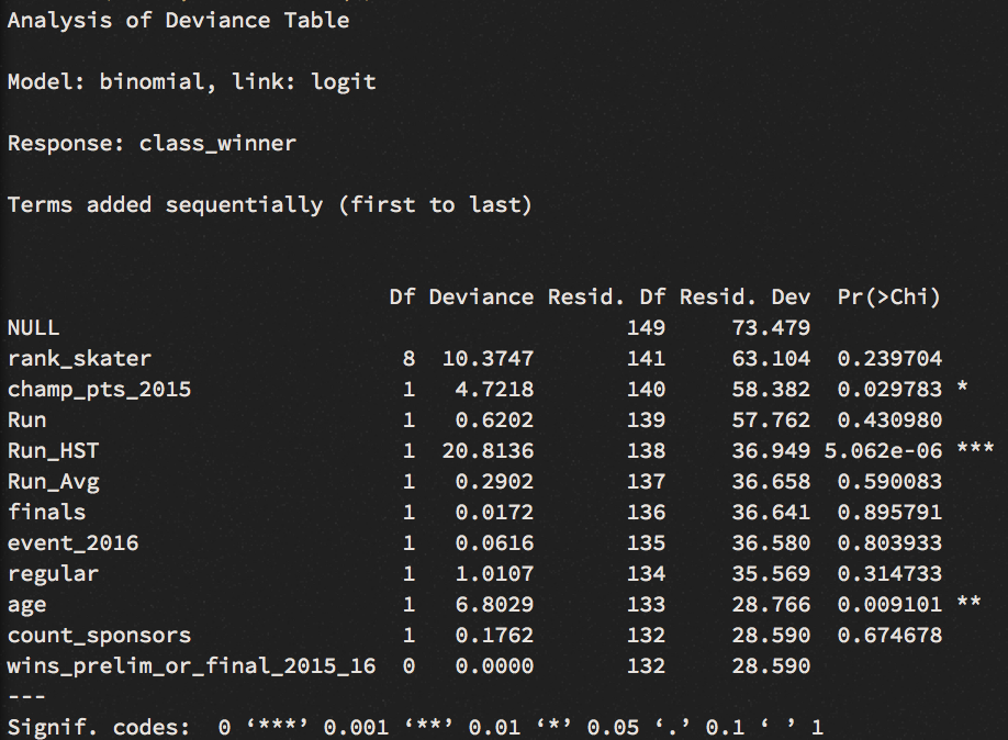
This gives us an idea on how well our GLM model performs agains the null model. Here we see that not only Run_HST reduced the residual deviance, but also the variables age and champ_pts_2015. For us it is important to see a significant decrease in deviance. Lets assess the model’s fit via McFadden R-Squared measure:

install.packages("pscl")
library(pscl)
pR2(model)

llh          llhNull     G2           McFadden    r2ML        r2CU
-14.2949557 -36.7395040  44.8890966   0.6109105   0.2586338   0.6678078

This yields a McFadden score of 0.611, which might be comparable to a linear regression’s R-Squared metric.

# Run on test data:
test_run<-test %>%
  select(-class_winner)

fitted.results <- predict(model,test_run, type='response')
fitted.results <- ifelse(fitted.results > 0.5,1,0)

misClasificError <- mean(fitted.results != test$class_winner)
misClasificError
print(paste('Accuracy',1-misClasificError))

#[1] "Accuracy 0.912280701754386"

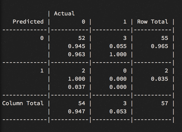
#CrossTable:
CrossTable(fitted.results, test$class_winner,
prop.chisq = F, prop.t = F,
dnn = c("Predicted", "Actual"))

While we get an accuracy of 91%, this result is misleading. The model couldn’t find who is going to win. Only who is not to win, which isn’t really our problem at this stage, but one reason we get such high accuracy score.

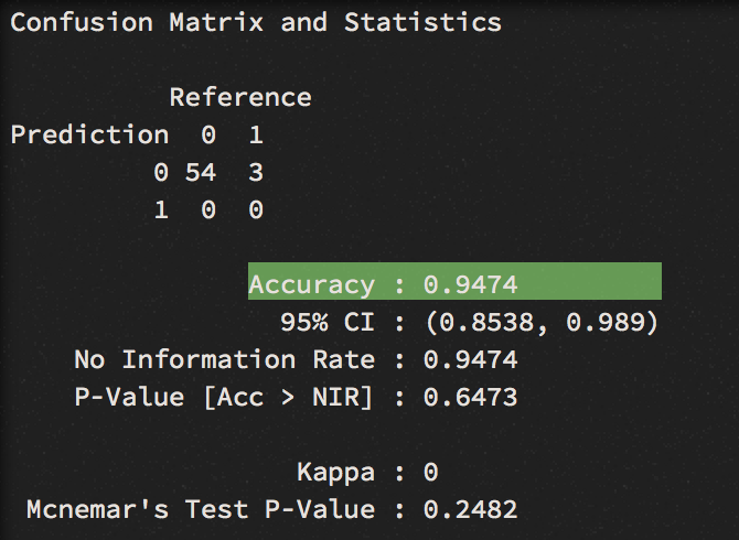
ctrl <- trainControl(method = "repeatedcv", number = 10, savePredictions = TRUE)
mod_fit <- train(class_winner ~.,  data=win_r, method="glm", family="binomial",
                 trControl = ctrl, tuneLength = 5)

pred = predict(mod_fit, newdata=test)
confusionMatrix(data=pred, test$class_winner)

We can confirm the accuracy result with K-Fold cross validation, a central model performance metric in machine learning. We apply one of the most common variation of cross validation, the 10-fold cross-validation and display the result via a confusion matrix. Now we get an even higher accuracy score of 95 percent. Still, the model couldn’t find the winners.

Predicting winning a medal:

The data only covers two years of the games. This makes it hard for a model like this to spot winners. What we could be doing instead is to tune down our standards, and only look for the lucky three winners who make it onto a podium. For that, we need to calculate an extra column, and add a “1”, for all skaters who made it among the top three, and “0” for the ones that didn’t. To test our new model, we will run it on the most recent game in New Jersey, after cleaning the training data.

set.seed(10)
win_r <- sample_n(test <- win[c(1:68, 77:207),], 199)

train <- win_r
test <- win[69:76,] ##New-Jersey-2016

model <- glm(top_3_outcome ~.,family=binomial(link='logit'),data=train)

test_run<-test %>%
  select(-top_3_outcome)

fitted.results <- predict(model,test_run, type='response')
fitted.results <- ifelse(fitted.results > 0.5,1,0)

misClasificError <- mean(fitted.results != test$top_3_outcome)
print(paste('Accuracy',1-misClasificError))

#[1] "Accuracy 0.75"

#CrossTable:
CrossTable(fitted.results, test$top_3_outcome,
prop.chisq = F, prop.t = F,
dnn = c("Predicted", "Actual"))

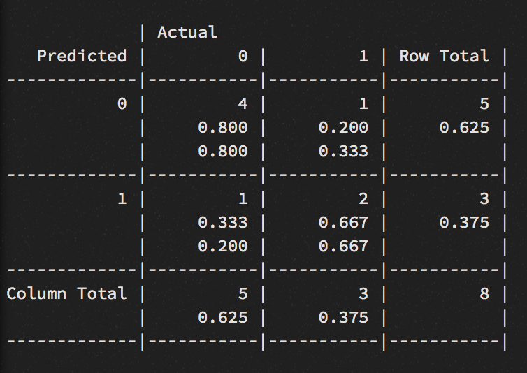
This model performs better. Except of 2 miss-classified instances, we got 2 out of 3 podium winners right. While it did well on the two winners - Nyjah Huston (1st), Chris Joslin (2nd), with 90% and 80% probability respectively - the model could not figure out the third place, that was labelled as “other” in our training data. Tommy Fynn was not included in the practice when I labelling the rank_skater column (skaters that will play Sunday’s finals were labelled in the data). As good practice requires, we will look at is ROC curve to produce a visual representation for the AUC, a performance measurements for a binary classifier.

install.packages("ROCR")
library(ROCR)
fitted.results <- predict(model,test_run, type='response')
fitted_for_ROCR <- prediction(fitted.results, test$top_3_outcome)
performance_ROCR <- performance(pr, measure = "tpr", x.measure = "fpr")

# plot:
plot(prf)

AUC <- performance(fitted.results, measure = "auc")
AUC <- auc@y.values[[1]]
#[1] 0.7333333

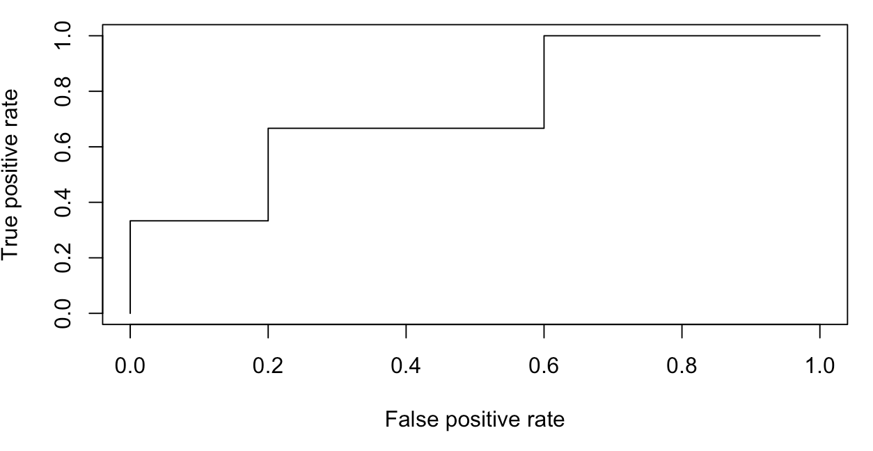
An AUC of 0.73 is not entirely pleasing, but it’s a start. We could now look for which score each skater on Sunday would need to gain for decent win probability. For this, we could build a test-set with the skater names and run scores ranging from 1 to 10 (we already know that skater and Run_HST are powerful predictors for the podium medals).

### probabilities for highest scores:
scores <- seq(1, 10, 0.1)

skaters <- c("NyjahHuston", "ShaneONeill", "PaulRodriguez",
             "LuanOliveira", "TomAsta", "RyanDecenzo", "CodyMcEntire",
             "ChrisJoslin")

df_skate <- NULL
for (skater in 1:length(skaters)) {
  for (s in 1:length(scores)) {
    df_skate <- rbind(df_skate, cbind(as.data.frame(scores[s]), as.data.frame(skaters[skater])))
  }
}

  names(df_skate)[1] <- "Run_HST"
  names(df_skate)[2] <- "rank_skater"

  fitted.results <- predict(model,df_skate, type='response') # with Run_HST and rank_skater as input variables

  ggplot(props, aes(Run_HST, fitted.results, group = rank_skater, col = rank_skater)) +
    geom_line() + theme_minimal()

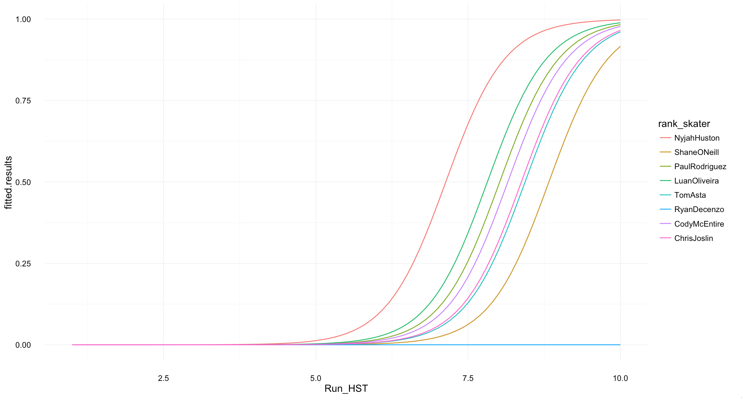
Win probabilities chart for each skater from their highest run scores.

Wrapping up

As we have seen, Nyjah Huston, Shane O’Neill and Paul Rodriguez do have best chances to make it on the podium. In which combination is unclear, but we will find out shortly. We have also learned how to apply a logistic regression on skateboarding, and how to compare the results across the various types of models we build. Two more models have been built. A neural network model and a random forrest model, both which didn’t perform as well as the logistic regression.